
原文發表於第 11 屆 iT 邦幫忙鐵人賽 (https://ithelp.ithome.com.tw/articles/10222248)
超級比一比之 CPM, FPKM, TPM
RNA-Seq 的主要目的之一就是找到試驗設計處理組間的差異表現基因 (Differential Expression Genes, DEG),這些基因之所以差異表現的生物意義再交由下游分析或是實際的分子生物實驗探討。先前已經介紹了 alignment-based 和 alignment-free 的轉錄產物定量工具,如:Bowtie2 和 kallisto,一個轉錄產物的定量結果可以用 counts per million (CPM) 來表示,這就是該轉錄產物豐富度的觀測值,下一步就是透過統計檢定了解該轉錄產物的豐富度在處理組間是否有顯著差異。統計檢定挑出差異表現基因這一步通常都可以透過 R 套件完成,例如 edgeR, DESeq2 等等。
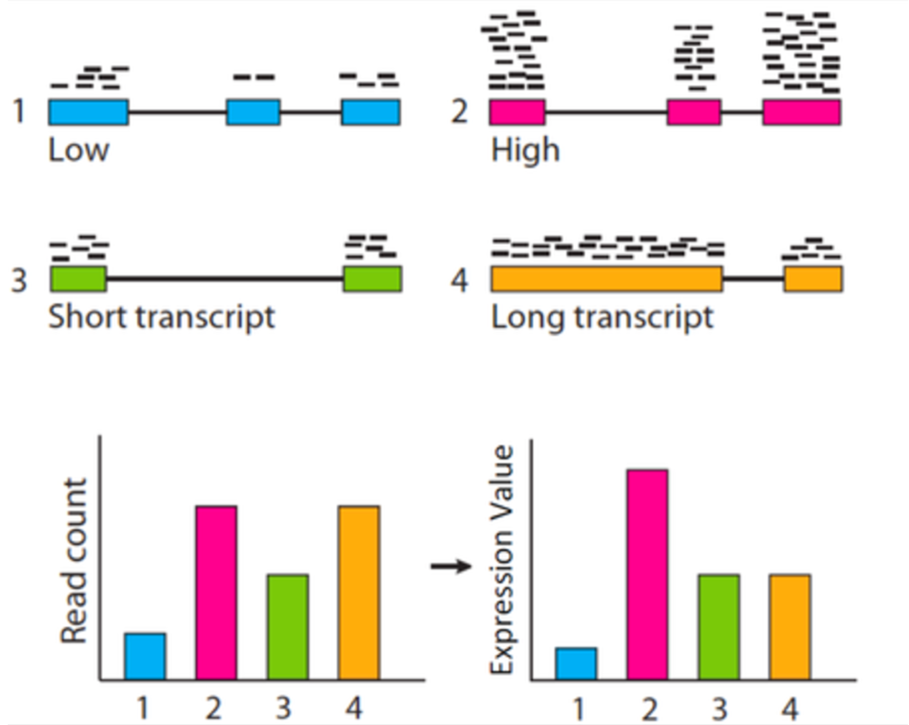
這邊要先提的一點概念是,統計檢定必須要以 CPM 來作為觀測值,而不應該是某些可能更常見的豐富度表示方式,如:RPKM (Reads Per Kilobase per Million), FPKM (Fragments Per Kilobase per Million), 或 TPM (Transcripts Per Million),這三種豐富度表示方式都是將基因長度考量進去的處理組內之標準化方式 (within normalization)。統計檢定要比較的是不同處理組間同一轉錄產物之豐富度,既然是同一轉錄產物之比較,便不需要將基因長度的性質引入標準化,任何多餘的資料前處理都是在引入偏差,這種情況對低表現量的基因影響較大!
 (看點療癒的東西放空一下,截圖來自龍貓)
edgeR 源代碼的部分
這邊貼上一段簡單的使用 edgeR 進行差異表現分析的腳本,輸入的 dd.csv 是 column 為不同處理組,row 為不同基因的表格,分析流程中包括了針對原始表現量的 PCA 分析、熱圖、差異基因篩選等等。改造自第一行註解中的原始碼,英文OK的朋友還是請直接到原始網頁中取得更完整的程式碼~
# 參考資料 https://gist.github.com/jdblischak/11384914
setwd("~/Desktop")
source("http://bioconductor.org/biocLite.R")
# biocLite("edgeR", dependencies = TRUE)
library(edgeR)
data_raw <- read.table("dd.csv", header = TRUE, sep = ",")
dim(data_raw)
head(data_raw)
tail(data_raw)
rownames(data_raw) <- data_raw$id
data_clean <- data_raw[1:(nrow(data_raw)), 2:(ncol(data_raw))]
#{r expr-cutoff}
data_clean
cpm_log <- cpm(data_clean, log = TRUE)
median_log2_cpm <- apply(cpm_log, 1, median)
hist(median_log2_cpm)
expr_cutoff <- -1
abline(v = expr_cutoff, col = "red", lwd = 3)
sum(median_log2_cpm > expr_cutoff) ##看看還剩下多少有過門檻
data_clean <- data_clean[median_log2_cpm > expr_cutoff, ]

# After removing all genes with a median log~2~ cpm below `r expr_cutoff`, we have `r sum(median_log2_cpm > expr_cutoff)` genes remaining.
# A good rule of thumb when analyzing RNA-seq data from a single cell type is to expect 9-12 thousand expressed genes.
# In this case, we have many more because the samples include RNA collected from many different cell types, and thus it is not surprising that many more genes are robustly expressed.
# **Question:**
#   What are some ways that we could improve this simple cutoff?
# What information are we ignoring?
# After filtering lowly expressed genes, we recalculate the log~2~ cpm.

cpm_log <- cpm(data_clean, log = TRUE)
# ```
# We can also explore the relationships between the samples by visualizing a heatmap of the correlation matrix.
# The heatmap result corresponds to what we know about the data set.
# First, the samples in group A and B come from very different cell populations, so the two groups are very different.
# Second, since the samples in each group are technical replicates, the within group variance is very low.
# ```{r heatmap}
heatmap(cor(cpm_log))
# ```
# Another method to view the relationships between samples is principal components analysis (PCA).
# ```{r pca}
pca <- prcomp(t(cpm_log), scale. = TRUE)
plot(pca$x[, 1], pca$x[, 2], pch = ".", xlab = "PC1", ylab = "PC2")
text(pca$x[, 1], pca$x[, 2], labels = colnames(cpm_log))
summary(pca)

## Two group comparison
# Now we start preparing the data for the the test of differential expression.
# We create a vector called, `group`, that labels each of the columns as belonging to group A or B.
# We then use this vector and the gene counts to create a DGEList, which is the object that edgeR uses for storing the data from a differential expression experiment.
# ```{r make-groups-edgeR}
group <- substr(colnames(data_clean), 1, 1)
group # 分組的代號
y <- DGEList(counts = data_clean, group = group)
y
# ```
# edgeR normalizes the genes counts using the method TMM (trimmed means of m values) developed by `r citet(c(Robinson2010="10.1186/gb-2010-11-3-r25"))`.
# Recall from lecture that the read counts for moderately to lowly expressed genes can be strongly influenced by small fluctuations in the expression level of highly expressed genes.
# In other words, small differences in expression of highly expressed genes between samples can give the appearance that many lower expressed genes are differentially expressed between conditions.
# TMM adjusts for this by removing the extremely lowly and highly expressed genes and also those genes that are very different across samples.
# It then compares the total counts for this subset of genes between the two samples to get the scaling factor (this is a simplification).
# Similar to normalization methods for microarray data, this method assumes the majority of genes are not differentially expressed between any two samples.
# ```{r normalize-edgeR}
y <- calcNormFactors(y)
y$samples
# ```
# The next step is to model the variance of the read counts per gene.
# A natural method for modeling gene counts is the Poisson distribution.
# However, the Poisson assumes the mean and variance are identical, but it has been found empirically that the variance in RNA-seq measurements of gene expression are larger than the mean (termed "overdispersion").
# So instead the negative binomial distribution is used, which has a dispersion parameter for modeling the increase in variance from a Poisson process.
# edgeR treats the Poisson variance as simple sampling variance, and refers to the dispersion estimate as the "biological coefficient of variation."
# Though it should be mentioned that any technical biases are also included in this estimate.
# edgeR shares information across genes to determine a common dispersion.
# It extends this to a trended dispersion to model the mean-variance relationship (lowly expressed genes are typically more noisy).
# Lastly it calculates a dispersion estimate per gene and shrinks it towards the trended dispersion.
# The gene-specific (referred to in edgeR as tagwise) dispersion estimates are used in the test for differential expression.
# ```{r model-edgeR}
y <- estimateDisp(y)
sqrt(y$common.dispersion) # biological coefficient of variation
plotBCV(y)
# ```
# The biological coefficient of variation is lower than normally seen in human studies (~0.4) because the samples are technical replicates.
# edgeR tests for differential expression between two classes using a method similar in idea to the Fisher's Exact Test.
# {r test-edgeR}

et <- exactTest(y)
results_edgeR <- topTags(et, n = nrow(data_clean), sort.by = "none")
head(results_edgeR$table)
results_edgeR
# How many genes are differentially expressed at an FDR of 10%?
# ```{r count-de-edgeR}
sum(results_edgeR$table$FDR < .1)
plotSmear(et, de.tags = rownames(results_edgeR)[results_edgeR$table$FDR < .1])
abline(h = c(-2, 2), col = "blue")
# ```
# As expected from the description of the samples and the heatmap, there are many differentially expressed genes.
# The [MA plot][ma] above plots the log~2~ fold change on the y-axis versus the average log~2~ counts-per-million on the x-axis.
# The red dots are genes with an FDR less than 10%.
# The blue lines represent a four-fold change in expression.
# [ma]: https://en.wikipedia.org/wiki/MA_plot
題外話之沒有重複怎麼辦
這邊來碎碎念一下一個有深切體會的問題,關於樣本的重複數。沒有錢送三重複的樣本去定序,所以一個處理組只送一個生物樣本去定序,這種情況在某些相對早期的探索性質的試驗上可能會出現。已經進行到定量完畢的分析流程,打算篩選差異表現基因,主流的軟體 edgeR 或 DESeq 卻不接受單重複的資料輸入請問怎麼辦?
其實沒有生物樣本重複,就絕對不能做統計檢定,也就是說其實完全沒必要使用上述的分析套件。能做的事情就是從上一步的定量結果,換算出 CPM 或 TPM 的數值,很直接地對數值進行闡述:Z 基因在 A 處理組中的豐富度高於對照組中的豐富度,B 處理組中的豐富度則比對照組低。分析者一樣可以自己定義一套標準,比如說將處理組除以對照組的豐富度之 log2 數值絕對值大於一就是差異表現基因,但是絕對不會有 p-value 跟 false discovery rate (FDR) 等等數值。
如果針對這個問題在網路上搜尋得夠久的話,還是可以在論壇上挖到一些秘招,比如說使用某幾版的 DESeq,搭配一些特殊的參數,就可以把單重複的資料丟進套件中,照樣得到有 p-value 跟 FDR 的報表。或者如果送定序時買的是某些公司的服務,就算只送單重複的生物樣本也可以得到上述的這種完整的有如有重複樣本般的神秘分析。這種情形有點自欺欺人的感覺,不是很有意義。但是考量某些情況下有些研究者為了生存所需還是會要做這樣的事情,所以還是在這邊簡單提上幾個關鍵字供參考。隨著次世代定序市場持續擴大,成本下降,希望這種單重複的問題可以逐漸在洪流中消失~如果手邊還卡著這樣的資料的話,別再猶豫趕快發一發,猶豫就會敗北~
 (在命運的安排下有時候還是會要做這種分析,截圖來自 JoJo 的奇妙冒險)
本身對於統計檢定並沒有太扎實的研究,不敢多言,僅提供簡單的腳本、基本概念及經驗分享,如果有任何錯誤之處或是想知道更多的方向,請不吝指教或留言討論~
參考資料與延伸閱讀
TPM data Differential expression analysis